Google Sheets Hacks: Conditional Formatting Uses

Google Sheets as part of Google Workspace, stands out as a versatile tool for businesses to manage, analyse, and visualise data. 

One feature that often doesn’t get enough credit or usage is conditional formatting. In this blog post and accompanying video, we'll explore the nuances of conditional formatting and show you five helpful hacks tailored specifically for Google Workspace users who may be unfamiliar with it, but also for those who do use it to brush up on its features!

The video has more detail on how these work, but below is an overview of how these could help utilise conditional formatting in your day-to-day or professional Google Sheets environment.

Top takeaways from this video:

• Find out what conditional formatting is
• Apply conditional formatting to a work or personal environment
• See some handy formulas that could assist your workflows
• Understand the formatting options
• Examples show how these work in real time

Understanding Conditional Formatting

Conditional formatting is not just a cosmetic tool; it's a robust feature that empowers users to dynamically format cells, rows, or columns based on specific rules. From basic text and date rules to custom formulas, Google Sheets provides a number of options to transform raw data into visually impactful insights.

Top 5 Uses for Conditional Formatting (with Examples)

Heat Maps for Trend Analysis

Mary, the Director of Guest Services at the Overlook Hotel. Mary employs the colour scale feature to create a heat map of guest numbers over time. By identifying patterns and trends, she strategically plans special offers during off-peak weeks, boosting engagement and revenue.

How to:

• Firstly she highlights all the guest number data from the fill icon, scrolls down to conditional formatting, and the conditional formatting menu slides out to the side
• From the tabs she selects colour scale and adds a colour to the minimum value point - red. 
• Next she adds a mid-point to visualise period that are on the cusp in cream 
• And lastly sets the max value point to white as a contrast colour 
• Once she clicks' Done' Mary can see that there are weeks in October & June where guest numbers are trending low, she can use this information to develop a special offer to drive interest in these quieter periods.

Highlighting Overdue Invoices

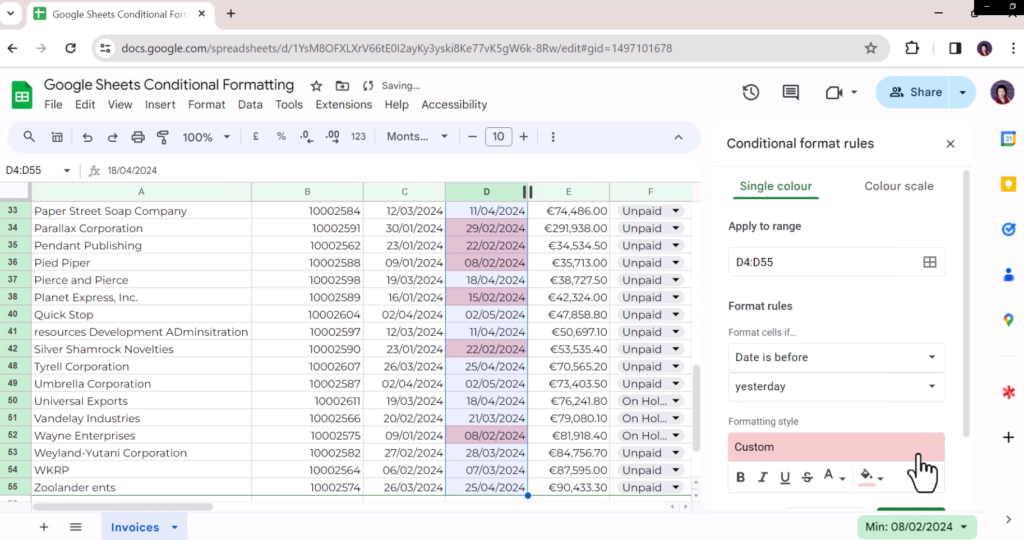
John, part of the collections team at Momcorp, leverages date conditions to swiftly locate overdue invoices. Applying a red fill to past-due invoices, John enhances efficiency in addressing payment issues promptly, ensuring a smoother financial workflow.

How to: 

• John highlights that data in Column D from row 4 down as this is the data which will drive his formatting. 
• Accessing the conditional formatting menu he selects “date is before” as a condition and yesterday as the target date. 
• John wants these invoice records to appear red so they are easy to spot, he clicks ‘Done’.

Finding Duplicates with Custom Formulas

In a learning and development environment, Noor uses custom formulas to uncover duplicate entries in feedback responses. By highlighting duplicate records in red, Noor reviews and analyses changes in delegate responses in detail, offering a nuanced perspective on training effectiveness.

How To:

• She is using a ‘COUNTIF’ formula to review the information found in Column B starting with B2. 
• She uses an absolute reference to the column to ensure that the formula is only checking column B and the greater than function telling the function to count cells if it finds more than one reference to the data in Cell B2
• She adds the custom formula  =Countif($B2:$B,$B2)>1   and selects a red highlight clicking ‘Done’ she can now review all the duplicate records in red before deciding whether to keep or delete them

Tidying Up Task Lists

Jill, overwhelmed with her task list for an upcoming sales event, seeks the expertise of Arun. Together, they create a conditional format to highlight tasks falling within the current week. This dynamic approach ensures Jill can focus on weekly priorities, streamlining her workflow and reducing overwhelm.

How to:

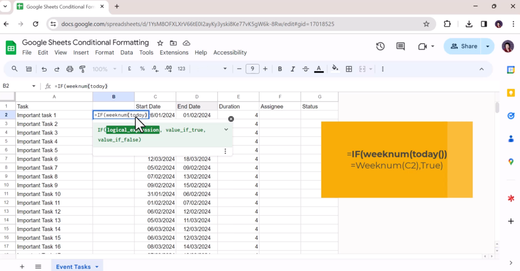
• Firstly Arun is going to add a new column, this will test whether the tasks start date falls within this working week. He does this by adding an ‘IF’ formula, this formula will test  if the week number for the date in column c matches the week number that corresponds with today's date. 
• If there is a match it will return a true statement in the cell. Once added Sheets offers an autofill to add the function in the cells below. We can now see a result for each task. 
• Now he needs to apply the conditional format rule to highlight the row. Arun selects all the data from Row 2 down, and navigates to conditional formatting.
• Selecting the 'Custom Formula is' option, in the custom formula box he adds the formula =$B2 which will pick up on and format any rows with a 'true' result.
• He can now hide the column testing the week numbers and the highlight will update weekly

Locating Weekend Sessions

Lile, a Shamrock Rovers player with familial responsibilities, utilises a custom formula to identify training and game sessions falling on weekends. By highlighting these sessions, Lile efficiently plans childcare arrangements, seamlessly balancing her sports commitments with family responsibilities.

How to:

• She highlights the information and accesses the conditional formatting menu, selecting 'Custom Formula is' she is going to combine a ‘WEEKDAY’ function (which looks for a particular day of the week) she is looking for Days 7 and 1  (It’s important to remember for this purpose that in Google sheets Sunday is day one of the week) 
• Then she adds an ‘OR’ function, remembering to wrap the Weekday functions in parentheses. This essentially creates a rule that reviews the dates in column A and highlights any that fall on Saturday or Sunday
• =OR(Weekday($A3)=7, (Weekday($A3)=1)) is the formula used to do this.

Customising Your Formatting Options

While default formatting options such as fill colours are widely used, Google Sheets offers extensive customisation possibilities. Users can experiment with hex numbers, RGB codes, and the eyedropper tool to create a personalised colour palette. Additionally, formatting options like bolding, underlining, italicising, and changing text colour can be applied to enhance data visualisation.

To conclude…

These five conditional formatting hacks represent just a small glimpse into the potential of Google Sheets. Whether you're uncovering trends, streamlining workflows, or conducting in-depth data analyses, mastering these techniques will undoubtedly enhance your Google Workspace experience.

Working with a Google Partner like Damson Cloud can unlock the potential within your business and tips like this can be found in our “Tip of the Week” program we deliver for clients, as well as clients working together with our Customer Success team who can increase productivity in your organisation by uncovering areas of improvement and supplying top-tier training.

If you think working with a partner would help you or your business, be sure to get in touch with us here and for more tips like this every week, subscribe to our YouTube channel!